Recap: Overfitting

• All data can be thought of consisting of two things:
  • Some generator process f(x) where x can be time or an actual input
  • Noise
• When we build model, we want it to learn only the generator process f(x)
  • The noise is random, it is unique to the training data
  • If we learn noise, results in overfitting

Choices to avoid learning noise: - Have simple model (few parameters) - Have more training data so that the network can avg out the noise

A single dimension parameter results with a straight line, 3 values will result in a parabola The point is that the higher dimension that we go, the more sophisticted the curve becomes.. This might results in fitting the data too well which includes the noise

Catch:

• A simple model may not learn f(x) well, underfitting
• The amount of training data needed grows exponentially with model complexity

If we tryign to learn a cube curve and we are using only enough parameters to learn a parabola, we will not get a good approximation.

Earling stopping point

• Stop when we see a certain state where it looks like it is overfitting

Drop out layer

• a fix percentage of neurons in layers are drop from training for one more epoch
• There are then put back in and another percentage are drop
• Reduce the num of training parameters

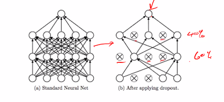
An epoch is one cycle through the training data

Problems:

• Drop too many neurons in each epoch: Underfit

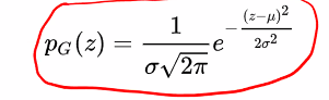
Noise layers

Add Gaussian noise to change the data to look like new data

Keras link

Regularisers

A penalty that is applied to the loss function of a layer

For example, in regresss our loss function may look like RSS (Square error loss):

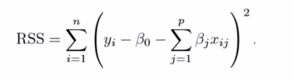
This will give us seuqared error

Our optimisation algo will find the values of params to minimise the loss function

• If there are too many para: the models starts to learn the unique noise of the training data – Overfitting or memorising
• Force a reduction -> Simplication -> In parameters

We can add in a penalty that is proportional to my parameters (l1 regulisation ) or Sequares of parameters (l2 Regulisation) to loss fnction:

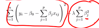
The hyperparameter lamda controls how much flexibility we give to the parameters, a higher lamba means more strict control

• L1: Eliminates less important parameters and simplifies the output
• L2: More effective in severe overfitting since it squares the parameters

If lambda is too high, the model will underfit

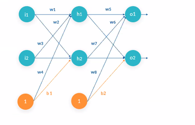
Regularizers

• kernal: Controls main weights (Lines connecting the green nodes)
• Bias: Controls the bias weights (Lines connecting the orange nodes)
• Activity: Controls based on layer outputs (o1 and o2)

Deep learning

In the previous lecture we look at neural networks:

• Unsupervised and supervised techniques
• Selection of hyperparameters
• Overfitting

The neural networks of the previous lectures has an issue:

• There will be many parameters to train
• Complex layers
• Curse of dimensionality

Trade of from learning ability and space

This is a motivation for deep learning

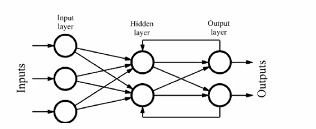
• consist of many layer
• Layers are not uniform
• Layers can have differnet function
• Transform and simplify the data so that networks at the end will be less dense and easier to use to train

Architecture: Long Short Term memories (LSTM)

Key issue with MLP:

• Assumption that samples are independent e.g the word ‘often’ usually follows ‘is’ or ‘are’. Words are not indepednent
• Solution: Use pas and sometimes future info to learn about current data

In RNNs we feed the output of the MLP back to the hidden layer and maybe backwards to previous layers

The prev output becomes the input for the hidden layer.

• Training is carried out using standard gradient descent that we talk abt
• If we unroll an RNN in time, we get:

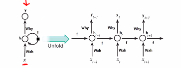
• We see that learning each new piece of data is now affected by past pieces

• Recurrent neural networks are good at learning from patterns in past data:
  • Predicting next words in sentence
  • Predict stock performance base on past data
  • Trajectory prediction forrobot
• Standard RNNS have probelm:

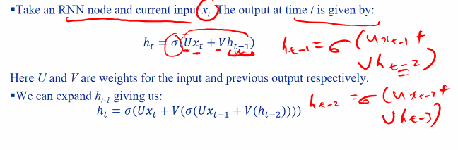
We will get this very long equation.. The problem here is that when we do our learning, we have to do our partial differential to get our weights. If we apply this chain rule, we will end up with a differential that looks like:

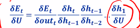
• The gradient of signoid is always small, as we multiply this gradient through time… it eventually gets 0
• When it becomes 0, it eventually stop learning

To Solve this, we introduce a special RNN called long short term memory

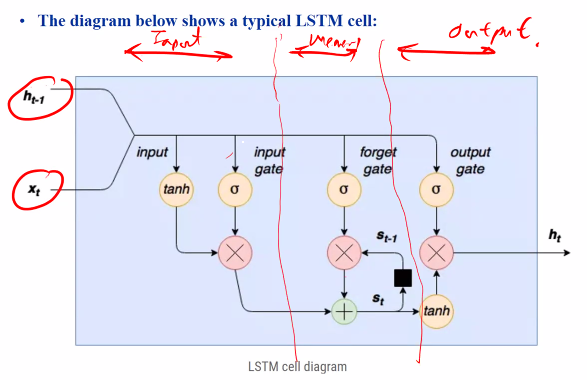
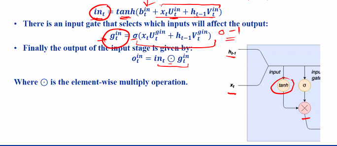
Input stage

• The inputs are multiplied by weights and put through a tanh function to squeeze it to betweem -1 and 1
• Input gate: Another neural network that is train to a value of 0 to 1, this controls the degree at which the input is allowed to pass to the next stage

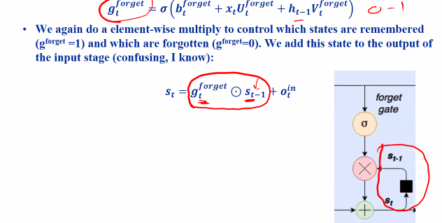
Forgot stage

• Forget gate: Learns the range from 0 to 1 and controls the influence of past and current input

Output stage

• Output stage: Decides what output to pass and what to suppress

Hidden layer size

• Each gate appears to be a single node but they are actually a collection of nodes
• The number of nodes in each gate is called the hideen layer size

Using the LSTM Cells:

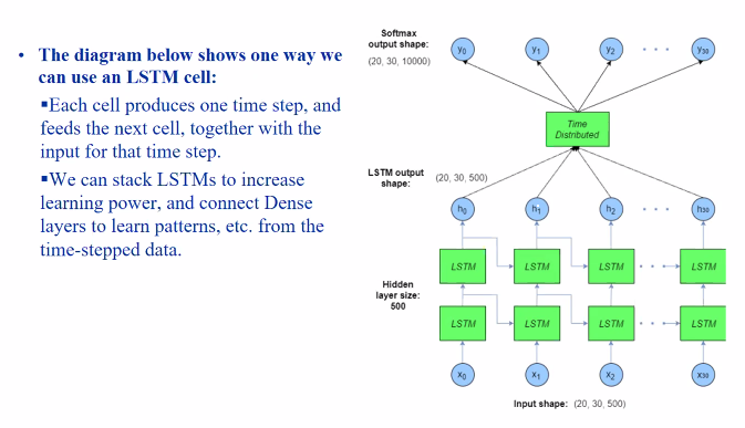
The network is one column, at the horizontal axis is the netowork over time.

• Takes the input
• Trains the LSTM
• Takes the memroy from prev time steps and train again and so on and so forth

Time distributed layer: Take the output over time and perform a classification or regression.

We can stack LSTM but

• More complex: More parameters

Using LSTM in Keras

{Check notes/slides 15 - 32}

Architecture: Autoencoders (AEs)

• Idea: Train a neural network to take an input x and generate the same output x. We will build a deep learning netwrok that does:

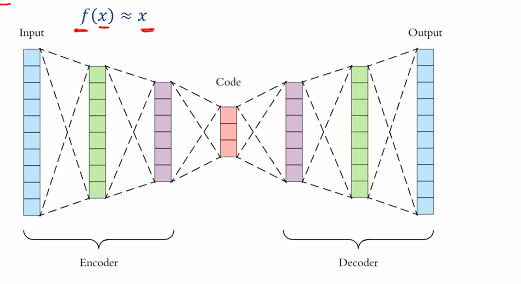
The stuff at the center is actualy the compress version of the input

• Achieving compression:
  • if the code layer is substantially smaller than the input, we can feed the input and use the resultant code as a compressed version of the input
  • We can feed this code into the decoder network to recover the original
  • AE however are very bad at this: recovered data will be highly lossy and the AE can only reconstruct data of the type it was trained on

But remember that because its a neural network, it is not really precise. (There might be some inaccuracy) Therefore the reconstructed data might be lossy (Noise and imperfection introduced)

• Detect anomalies:
  • When AE sees typical data it was trained on, it can reconstruct the input with minimal error
  • When the data becomes atypical, reconstruction error rises. We can flag anomalies when this error exceeds a threshold.

Autoencoders are very good to spot defects in teh system

Simple

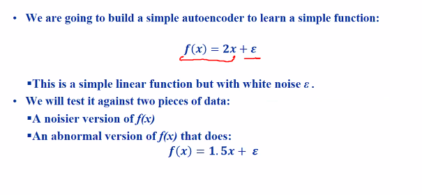
• F can be our throttle position sensor
• Train the neural network to guess the acceleration base on the position of the trottle position

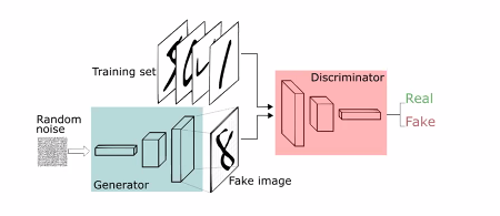
Architecture: Generative Adversarial Netowrks (GANs)

Motivation:

• Often dont have enough training data
• Want to build a neural network that will produce fake data from real data

Consist of:

• A generator network that learns how to counterfeit the data
• A disciminator networks that learn how to differentiate betweem the real and fake data
• We can use GANs to do things like: Producing images of people who dont exist

What are they

• Generator:
  • Random noise is presented to the generator
  • The generator uses this to create its fake data
• Discriminator
  • both fake and real data are presented to the discriminator
  • discriminator is trained how to differentiate them

How do they work

• Training generator
  • Weights for discriminator are frozen
  • The GAN is trained of the assumption that the fake data is real
  • End result: The generator adjusts its weights to try to maximise the realness of the fake data
  • The process repeats
• Training alternates between:
  • Maximising the discriminator ability to tell fake data from real
  • Maximising the quality of the fake data to minimise the discriminator ability to differentiate

This is why it is called an adversarial networks as both netoworks try to fight each other

• We are trying to trick the discriminator that it is real
• The generator has to then try to generate better fakes

Generating

{Check notes 48-56}

Training

• Create generator, discriminator and GAN networks and load the data
• In each epoch for discriminator
  • Generate fake data using random numbers
  • Randomly choose real data and combine with fake data
  • Tag the real data with 1 and fake with 0
  • Train the discriminator
• In each epoch, for the generator
  • Freeze the discriminator weights (The discriminator does not become smarter)
  • Generate the fake data using random numbers
  • Train the GAN with the assumption that the fake data is real
  • This forces the generator to optimise its weights to maximise its score from the discriminator
  • the discriminator itself is not affected since its weights are frozen

See slides for epoch example 1) Take as input of the generator and discriminator 2) Create input layer 3) Pass the input layer over to the generator which will produce an output 4) Use this output as the input to the discriminator 5) The output from the discriminator would be either true or false (Real or fake)

To reduce the lost, we have to make the generator generate better data that tricks the discriminator

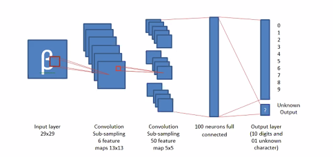
Architecture: Convulutional Neural Networks (CNNs)

Traditionally used to for image recogntion or be use for other stuff like sequences.

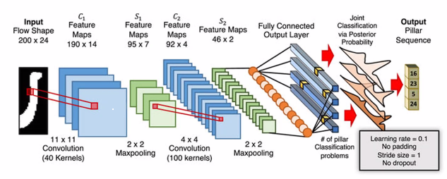
• Convolution kernal scans the image and produce a feature map
• We can have many conv filter and each filter will produce a feature map
• The end result is we will have alot of feature maps
• our feature maps will either be the same or larger than the image
• We will do pooling to summarise the data
• From the output we will filter again and result with another set of feature maps
• This will repeat

Standard dense multilayer perceptrons (Classficiation)

• Use softmax

Convolution layers

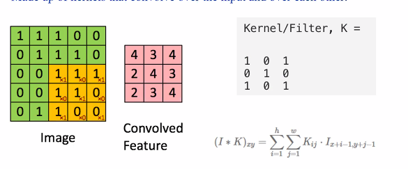
• Yellow window: Filter
• Green: The original image

The yellow window will travel over the image

The CNN primary distinguishing feature is the convulution layer. - Made up of kernals that convolve over the input and over each other

The depth of the kernal is equal to the depth of the data.

• E.g with colour images, there are 3 channels and the kernal is 3 layers deep:

For colour image:

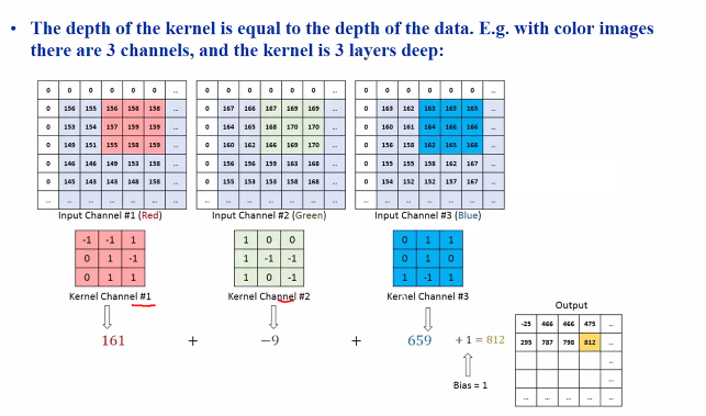
• The kernal function as feature extractors and the output from the convolution operation is called a feature map
  • As training progresses the kernals become optimised to extract key infomation like edges, repeating patterns, etc in input data
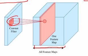
• Many kernals can be use on one layer
  • This will produce a volume of feature maps instead of a single feature map
  • Due to the randomness of the initial kernal, each feature map ends up extracting a different feature of the input.

They treat the kernals as weight and apply gradient descent on the kernal.

• You can convolve kernals over earlier kernals
  • The feature maps generated will represent higher level features of the input
  • E.g the lower kernal might extract lines, the higher kernal might extract shapes

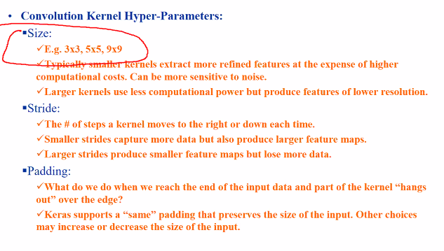
Parameters:

1. Size

Choosing kernal size:

• Smaller: More refine but more computation cost and might be more sensitive to noise
• Larger: Lower resolution but less expensive

1. Stride
   • The number of steps the kernal moves to the right or down
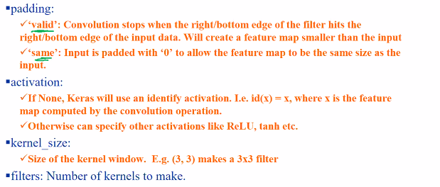
2. Padding
   • Decides what to do when we hit the end of the image
   • Can choose to let the kernal hang out outside (Convoluted to the last square)
   • Feature map will be the same size of the image - Same padding: Allow part of the kernal to hang outside the image so that we can convolute outside the kernal

Layers:

• Padding
• Activation
• Kernal_size
• filters: How many kernals to make

Pooling layer (To do a Summary)

• The pooling layer takes a nxn region of the feature map and either picks the max of takes avg

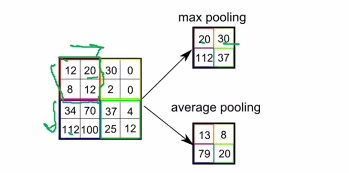
• pooling layers:
  • reduce dimensionality and hence computing power: a 4 by 4 can go to a 2 by 2
  • Extract the most dominant featueres (Max pool): Gives the model shift invariancy and less sensitvie to noise
  • Averages the features

Hyperparameters:

• Stride : How many pixels to jump to the right and down
• Size: Dimensionality of our max pool
• Keras pooling
  • Pool size: The length or dimension of the pool
  • Strides

If our stride is our max size, our feature map will reduce by 1/size in each dimesnsion

Generally the first few layers of the CNN consist of alternating convolution and pooling layers

• BUT, stacking to many pooling layers can result in loosing all data

Flatten layer

• Convert the 2d feature map into a 1d vector
• This will go into a standard multilayer perceptron
• My output would have many classes

Slides