Advantages
- Statistical methods have better theretical
- Statistical methods in general are faster to build and train
- Statistical methods usually have fewer hyper parameters to adjust
Statistical - Linear Regression
We have data that shows the relationship between a dependent variable and one or more independent variables
e.g The relationship between population growth and time
- Relationship between the dependent variable and the independent variable can be a straight line (Linear) or not (Nonlinear, ie curve)
- Consider linear relationship with one independent variable (Simple linear regression)
- Previous lecture we build regression model using gradient descent
- Our model will be based on equation of a straight line
Good example of how statistical methods have better theoretical basis than neural networks
- Our model will be based on equation of a straight line
Simple linear regression
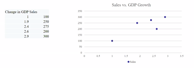
- Independent variable: Uncontrollable variable. (GDP growth)
- Dependent variable: The variable that we are interested in predicting agaisnt the independent variable. (Sale)
The in
Assumptions
- There exist a correlation between dependent (y) and independent (x) variables
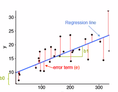
- y depends on x through a linear equation:
yi = a . xi + b(Blue line) - We add a random noise e in the observation
yi = a . xi + b + ei - Our task
- Test if there is a relationship between x and y
- Find a and b
We are trying to make a relationship so that we are able to predict the future
Covariance
If there is a change in one variable when the other variable change, this is a covariance
Example
- (Xi - X) shows the difference between both pointss value will be large
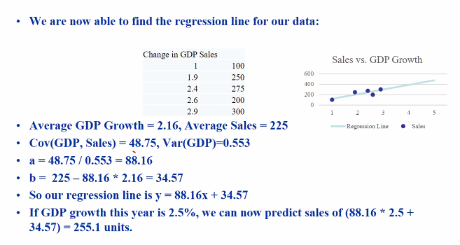
Calculating the avg for the GDP and Sales figures:
- Avg(GDP)
- AVG(sales)
- Cov(Sales, GDP)
If COV is positive, sales figure grow in the same direction as GDP
We know that there is a correlation but we dont know if the relation is strong.
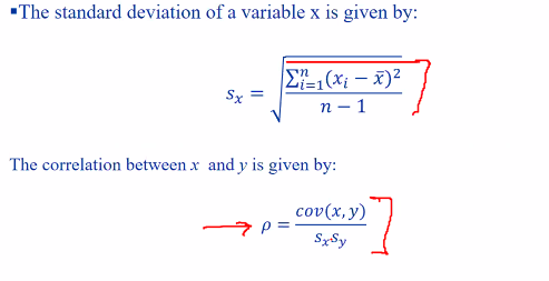
Correlation
Correlation will give us a better idea of the relationship. Correlation will scale our values from -1 to 1. This will allow us to determine the strenth of the relationship
- If the value is close to 1, we can see that the figures are strongly related
Parameter estimation
yi = a . xi + b + ei
- The error is therefore:
- ei = yi -a . xi - b
- Lost function:
This gives us an idea on how good our model is.
-
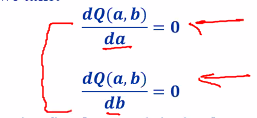
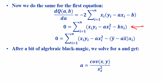
To minimize Q(a,b), we take:
-
Doing the second equation
Solve for b
- Setting it to 0 and solving for b we have
- b = ySIGMA - a . xSIGMA
This makes sense because our avg are going to be dependent on both x and y. Therefore the avg will restrict on where the intercept is
Example
Even thou we got 255.1 unit, this is just a rough estimation due to the noise
Naive Bayes Classification
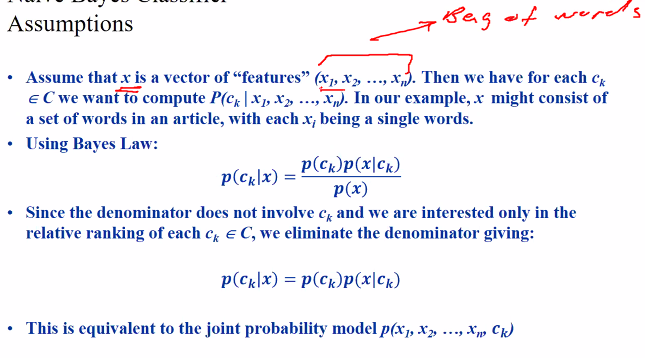
Given a set of data X and a set of class C, we want to compute the likelihood of some x in X belongs to some class in C
Examples
- X is a set of news article and x is a article
- C is a set of news article types e.g sports, politics
- Our task is then to decide what kind of article x is
Assumption
- Each vector represent a word.. we want to see the frequency of the words.
- But theres a problem because it does not consider the order of words
- This could cause error because sometiems order of words are important > This is where we get classiification error
Using Chain rule:
we are looking at the probability of some xi given xi+1…etc
We take the naive assumption that all these values occur independent of each other. (This does not make sense in normal english) e.g “Joint probability” happens more often compared to “final joint”
Parameter estimation
- Uniform: For n classes, the probability is simply 1/n
- Base on training set: There is a total of S training samples and sk samples for class ck, then p(ck) = sk/S
Estimation assumption:
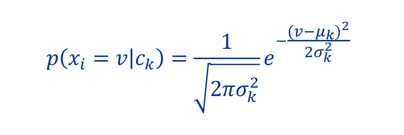
- Gaussian: Assumes that the probaility of a feature xi taking a particular value v in class c follows a normal distribution
- Good for linear values
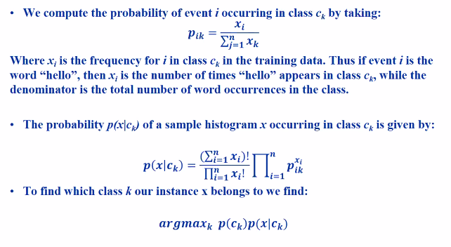
- Multinomial: Assumes thaat the frequency of a feature xi occuring in a class is govenred by a multinormial distribution
- Good for frequency
- Bernoulli: Assumes that the boolean occurance of a feature xi occuring in class ck is govenerment by a Bernoulli distribution
- Good for binary
Continous variables
- Classes contains continous variables
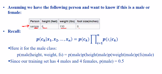
- E.g when classifying male and female, we may just consider height, weight etc
Example
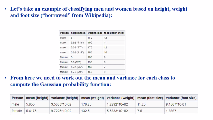
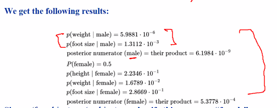
We use a gaussian distribution here.
- Since our training set has 4 male and 4 females, p(male) = 0.5
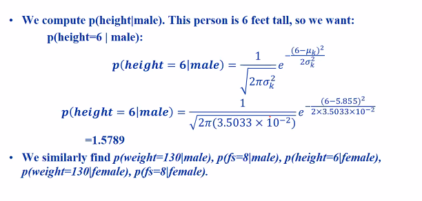
Because the p(female …) > p(male ..), we can conclude that this person is “female”
Naive Bayes - Multinomial
Issues
- Raw frequencies in document classification face some problems
- Bias towards longer documents
- Bias towards connector words such as “the” because they occur more frequently
We try to fix this by using tf.idf (term frequency inverse document frequency):
Adds a small number to it such that the word that occur many times in document will get a punishing term. (Total number of documents / Documents containing the word i)
- Zero frequency
-
Pik = 0 and P(x ck) becomes 0 - Laplace smoothing: Add 1 to every xi so that it wont be 0
-
Naive Bayes - Bernoulli
Sometimes we are interested if the event even occurs at all.
No. of times it occurs / Samples
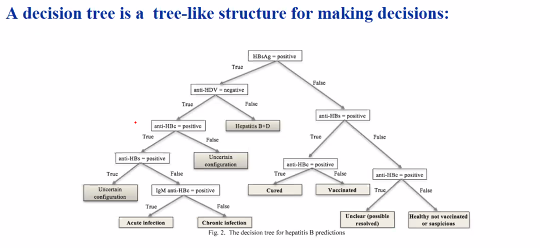
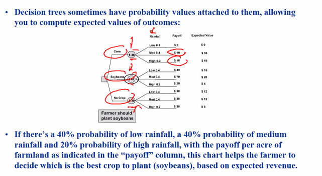
Decision trees
Classification to be explainable or calculate on the expectant values
Appealing because:
- easy make decisions
- Provides a way to explain decisions
Example
- If too much water, plant die
- If too little, plant die
- Just nice.. good for farmer
Deriving trees
- Guesswork based on expert opinion
- Based on historical data
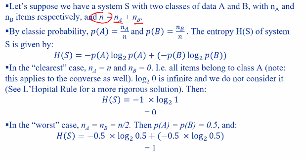
Entropy: Amount of uncertainty in a data
The entrophy is 1 which is the worse case if its evenly distributed
We will use ID3 algo to generate the tree
ID3 algo
- Choose a decison criterial that reduce uncertainty as much as possible
-
p(x) = nx / n and H(S A) is the entropy
Example
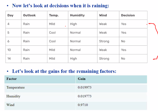
- We want play tennis
- We need to see weather outlook, temp, humidty and wind to decide
- Looking at bob;s pattern of decision making and try to learn
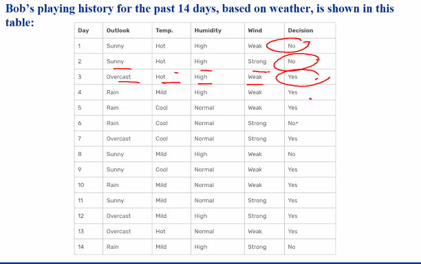
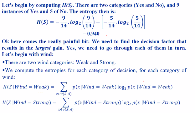
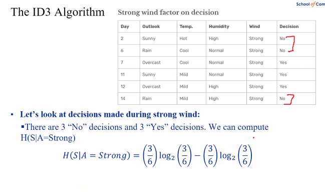
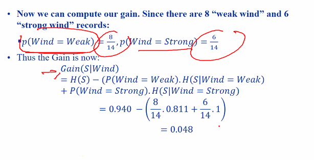
We have to go through each of the decision factors in turn
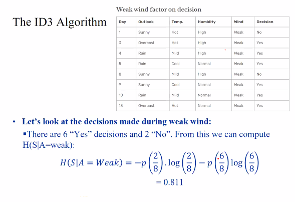
| p(x | Wind=weak) : Probability of yes or no given wind is weak |
We can find our entrophy base on the decision made after making the graph smaller.
The entrophy here is 1
Therefore
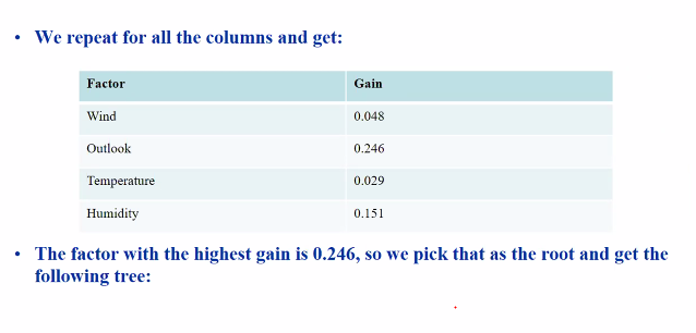
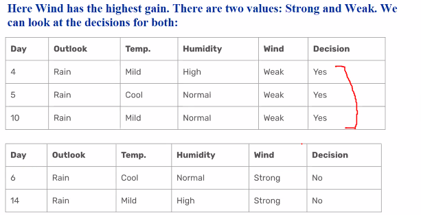
We have to do this for the other graph and pick the highest gain
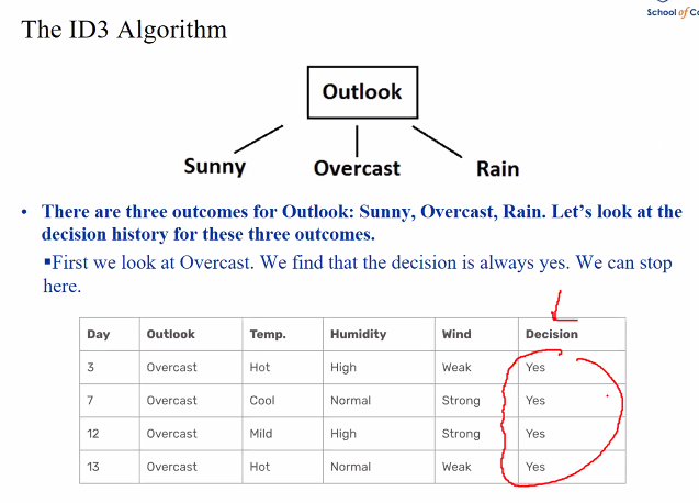
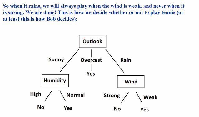
We will get the tree:
Repeat this for the other variables such as humidity/Wind/Outlook
Look at wind:
The final tree after finding all:
We start from the largest gain and go downwards
Drawbacks
- It only works with nominal values (factors has values that are clear categories)
C4.5 actually addresses it by take the discontinous ranges and chunks them into bins
Decision trees can also be use for regression
Support Vector Machines
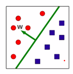
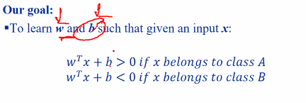
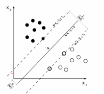
A hyperplan is a d dimennsional plane defined by its normal vector w
- in 2D, a hyperplan is a strightline
- normal w is orthogonal to all points on the plane
- The hyper plan seperates the d dimensional space into two halves
- Hyperplanes always pass through the origin
	> This restricts its ability to partiiton the space
	> To fix this we add a d-dimesnion bias b
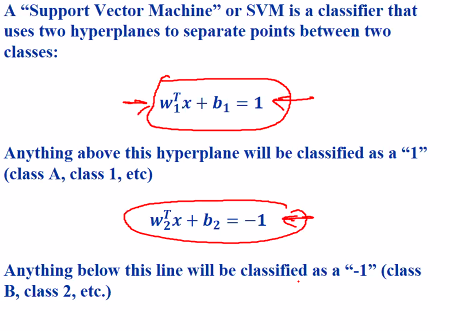
Assumption
The lines will pass through points closerst to the center, whihc is why they are called support vectors
- These two hyperplanes must be far apart as possible
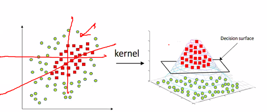
Non linearly sperable points
Some times we cannot draw a line no matter what you do:
So we run a kernal trick which change to a 3D plane which becomes a decision surface.
Configuration
Loss function:
- Hinge loss: Useful for linearly sepearble classes
- Logisitcs: Probability estimates
- Perceptron: Uses loss function
- Modified Huber: Outliers
Training rate: Controls how fast the svm learns
- High value: Fast but poor learning outcome
- Low: Slow training
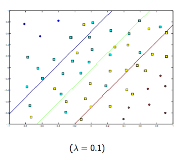
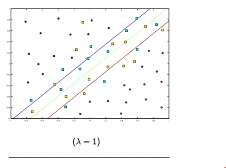
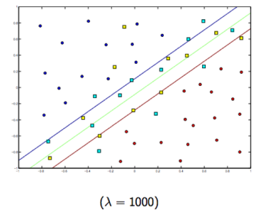
Regularization: Controls how we penalized misclassified
- Higher penalty:  Underfitting : SVM performs poorly even on training data
- Lower Penalty: Possibly more overfitting: SVM can only understand and correclty classify training data
The more para, the hgiher chance of getting overfitting
- L1 : Adds a penalty term that use the Absolute value of the model parameters, results in model with fewer parameters
- L2: Adds a penalty term that uses the square of the value of the model parameters, results in Compact denser models
- Elastic: Both L1 and L2 combine
