Hypotheses testing base on normal distribution
Null and alternative hypothesis
-
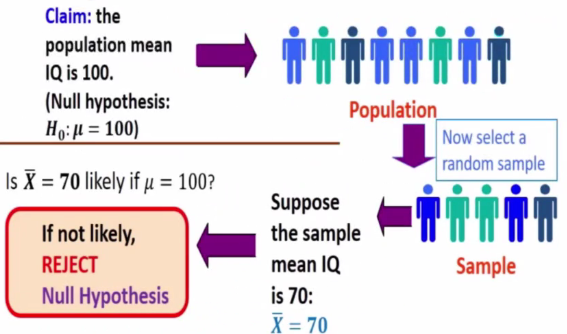
A statistical hypothesis is an assertion on conjecture concerning one or more populations
- Consider 2 characteristics of a population
- Ratio
- Mean
- Variance
- “do not reject” and reject
Statistical hypothesis
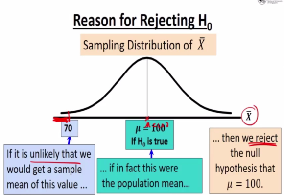
The rejection of a hypo is to conclude is false
Acceptance of Hypo implies that we have insufficient evidence to believe otherwise
Because of this terminology, the statsician will often choose to state the hypo in a form that hopefully will be rejected
Null hypothesis
- Denoted by H0
- Fomulate in hope of rejecting
- Concern a population parameter will always be stated to specify an exact value of the parameter
Alternative Hypothesis
- Denoted by H1
- More than one values
- Rejection H0 this leads to the acceptance of alternative hypothesis denoted by H1
E.g 1
- We want to determine if the mean of IQ of pupils in a certain sch is different from 100
- We have H0: u = 100 against H1: u != 100
This is call two side alt
Type 1 and 2 error
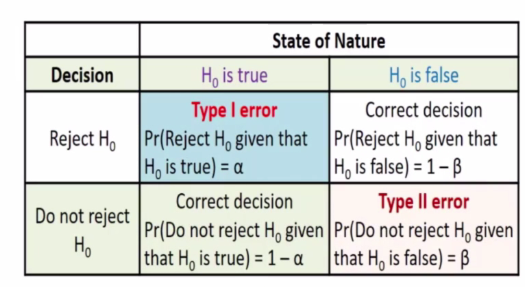
Type 1: Reject the null given that it is true Type 2: Do not reject the null given that it is false
Type 1 is a serious error
- Probability of committing a type 1 error is 5 percent or 1 percent, this is also known as level of significance
Type 2 is beta
Acceptance and rejection region
- Select a suitable test statistic for parameter under hypothesis
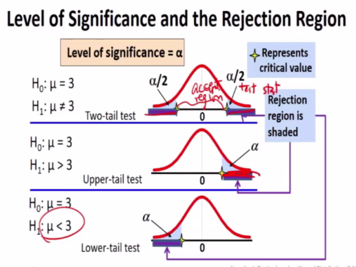
- Once the sig level a is given, a decision rule can be found such that it divides the set of all possible values of the test statistic into two regions
1) Rejection region/critical region
2) Acceptance regions
The value that seperates the rejection and acceptance region is called critical value
E.g 1
- A certain type of vacchine is known to be 25 percent effective after 2 years
- To determine if a new and more expensive vaccine is superior (Can protect for longer time)
p of origin = effective = 0.25
If we want to be superior, we must have p>0.25
- 20 people choose at random and use new vaccine
- If more than 8 of these people surpass the 2 year period, then the new vacchine will be considered superior to the one presently in use
X = num of individual out of 20 that surpass the 2 year period without contracting the disease
This is consider a success
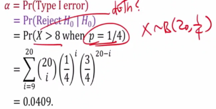
This is equivalent to test H0 = p = 1/4 and h1 = p >1/4
We reject H0 when X > 8 when p = 1/4
Follow binomial distribution of X~B(20,1/4)
This means that chance of getting type 1 is 4 percent
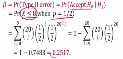
But we want to ask what is the probability of committing of type 2 error?
- We cannot compute unless we have a Specific alternative hypothesis
If let say p = 1/2
Chance of not committing an error is 1-beta = 1 - 0.2517 = 0.7483
This is vert good because the chance of not commiting the error is very big
Hypotheses testing concerning mean
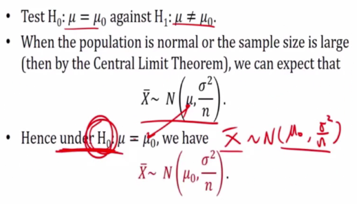
Consider the problem of testing the hypo concerning the mean.
Considerations:
- Variance is known
- Underlying distribution is normal or n is very large (>30)
We are going to look at the difference to tell if its big or not.
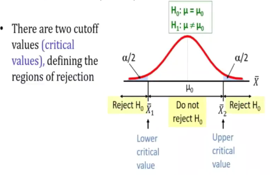
Two sided test
Critical value approach
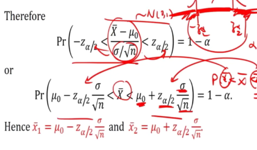
We will try for the interval of Xspa where
x1spa < Xspa < x2spa defines the acceptance test
p(x1spa < Xspa < x2spa) = 1-a
We will put xspa at one side of the inequality
- Reject when Xspa is between x2spa and x1spa
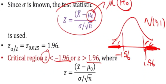
- Critical region is usually stated in terms of Z rather then Xspa
However, we can represent it as a t distribution
E.g 1
- Breaking strength 35 kg
- SD is 1.5 kg
- Determine if breaking machine has those stats
- Random sample of 49 piece
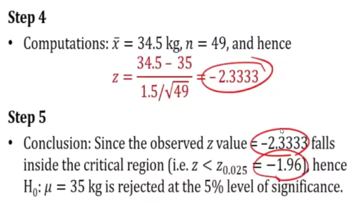
- Mean breaking strength of 34.5
-is there evidence that the machine is not meeting the specification for mean breaking strenrh
Letting u be the mean breaking strength by the machine
1)
h0: u =35 h1: u !=35
2) Set a = 0.05 (Not stated in question)
3)
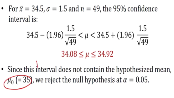
Relationship between 2 sided test and confidence interval
-
The two sided test procedue just describe is equivalent to finding a (1-a)100% condifence interval for u
-
H0 is accepted if the confidence interval covers u
-
If the C.L does not cover u0, we reject u = u0 in favour of the alternative H1:u!= u 0
Critical value approach and p-value approach
P-value approach to testing
Pvalue: probability of obtaining a test statistic more extreme than the observed sample value given H0 is true
This is called observed level of significance
The level of significance is fixed
If our test statistic falls out of the bounds, we reject.
What is the chance that we commit a type one error?> This is level of significance
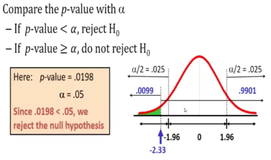
- Compare the p value with a
. Extreme case: Larger than observed
E.g 1
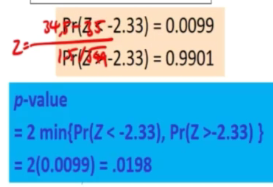
- How likely to see a mean of 34.5 if true mean is 35
- muel = 1.5
- n = 49
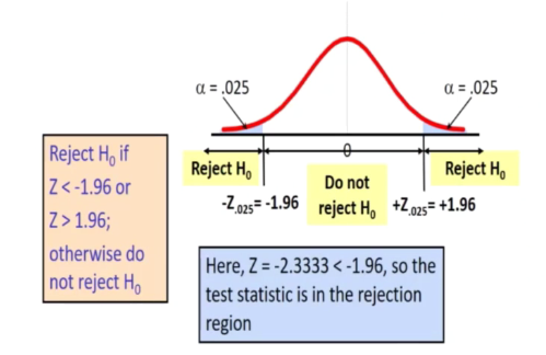
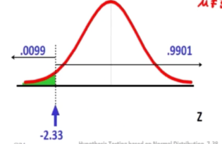
Xspa = 34.5 is translated to a Z score of -2.33
Rejected
One sided test
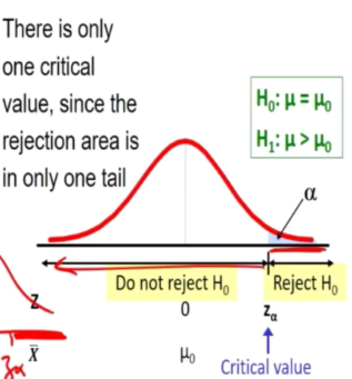
H0 is rejected if the observe values of Z is greater than Za

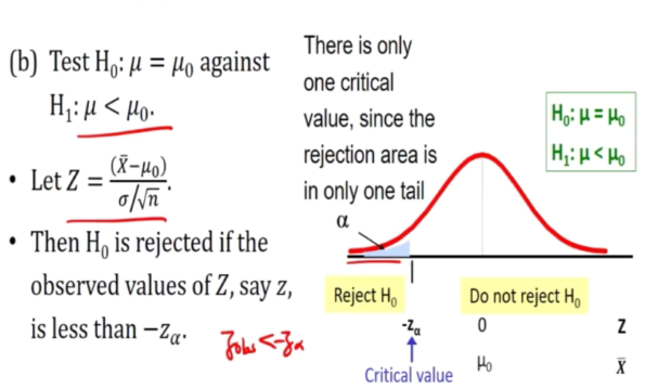
b) Test h0: u = u0 against H1: u< u0
E.g 2
- Sports equipment fishing line
- Mean breaking strenth is better than the Market avg strenght of 8 kilo
- Suppose breaking strength has a sd of 0.5kg
We have to look to evidence to show that u is different
-
Random sample of 50 test to have mean of 8.2kg
-
Use 0.01 level of significance
1) Let u be mean breaking strength of the new type of fishing lines
H0: u =8 against H1: u>8
2) Set a = 0.01
3)
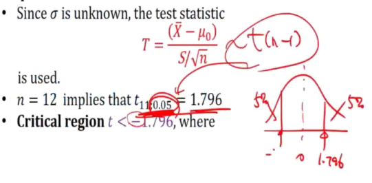
Since sigma is known,
Follows a normal distribution.
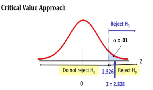
Za = Z(0.01) = 2.326
Critical region Z > 2.326 where
4)
5) Since the observe falls in the critical region (2.326) and z is 2.828.
Hence H0: u = 8 is rejected at 1 percent level of significance
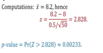
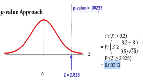
Conclusion based on p value since pvalue ~ 0.00233 is less than 0.01 hence H0 is rejected at 1% level of significance.
Hypothesis testing on mean with variance unknown
- We do not know sigma
- We can guess it
1) Variance is unknown 2) Underlying distribution is normal
E.g 3
- The avg length of student register for summer classes at certain college been 50 minute
- New registration procedure is being tried
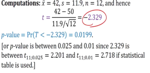
- Random sample of 12 students have avg reg of 43 minutes with a sd of 11.9 minutes under the new system
- Test the hypo that the population mean is now less than 50 using level of significance of 0.05
Indentify that 50 is the old one and that u is the avg time for the new procedure
We are trying to test for u = 50
Xspa = 43
S = 11.9 (Standard deviation)
a = 0.05
[Note] If this was not normal, we can only use this method if the sample size is super big
Let u be mean of new procedure
H0: u=50 against H1: u<50
We do not have that variable in our T table, we use estimation, we do not need the exact p value
- Reject the null hypo since observed value t = -2.329 falls inside the critical region t<t0.05: t = -1.796
Do we reject the null hypo if our a is above 1 percent but below 2 percent
-> We do not reject
Hypotheses testing concerning difference between two means
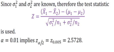
1) variance of 1 and 2 are known
2) underlying distribution is normal or both n1 and n2 is very large
E.g 1
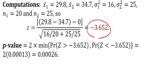
- n1 = 20
-
Avg yield x1 = 29.8
- n2 = 25
- Avf x2 = 34.7
- Assuming that the strength distribution are normal with sigma1 = 4 and sigma2 = 5
- Does the data indicae that the corresponding true avg
Let u1 and u2 be mean strength

Thus it is rejected
Large sample testing with unknown variances
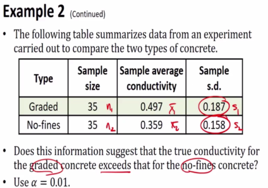
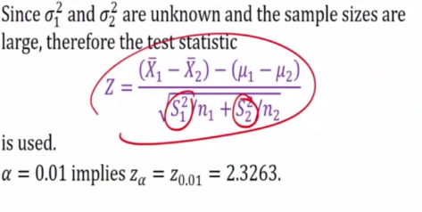
- Because it is large, instead of sigma1 ^ 2, we replace by s1^2
- We can see that it is approximate normal
E.g 2
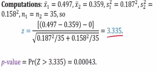
Anything bigger than Z is rejected
Therefore we reject since z = 3.335 falls inside the critical region.
Unknown but equal variances
What if we do not know what they are but we know that they are equal?
If the sample is big, we have a better estimate, therefore we take the bigger.
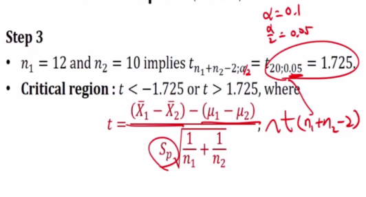
1) Variances are equal but unknown
2) Pop are normal
3) Small sample size
If the sample size is big,
E.g 3
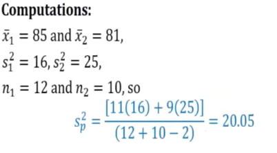
- Math was taught to 12 students for one group
- Anotehr group of 10 students same course by program materials
-
At the end, they all sat same exam
-
Test the hypo that the two learning methods are equal using 0.1 level of sig
- 12 students avg 85 sd 4
- 10 students avg 81 and sd 5
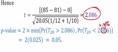
H0: u1 - u2 =0 against H1:u1-u2 !=0
We reject the null hypo since t is 2.086 which falls inside the critical regiion
H0 : u0 = u2 is rejected
Paired data
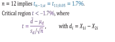
E.g 4
- Do data provide sufficient evidence that method 2 yields a higher avergae percentage than method 1?
- Assume difference are normally distributed
- Use a = 0.05
We are looking for big difference (T>t)
1) H0: ud = 0 against h1: ud<0
The reason for this is because we are d = x-y = u1 - u2
3)
4)
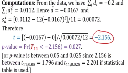
We do not have the exact value for 2.156 but we have 1.796 and 2.201 using statistical table.
5)
Rejected
Hypothesis testing concerning variances
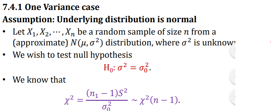
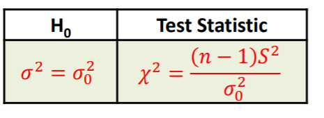
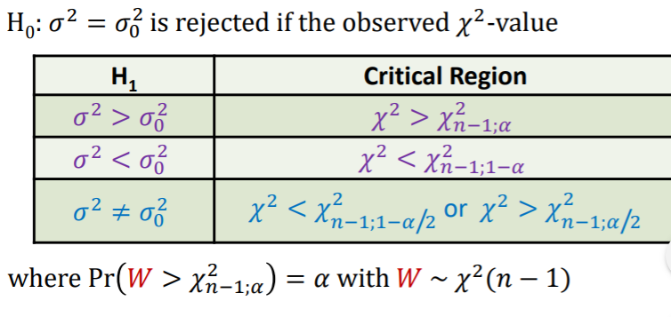
One variance case
Assumption: It is normal
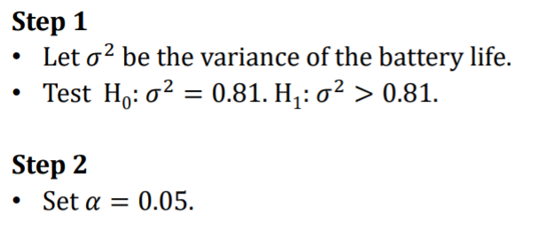
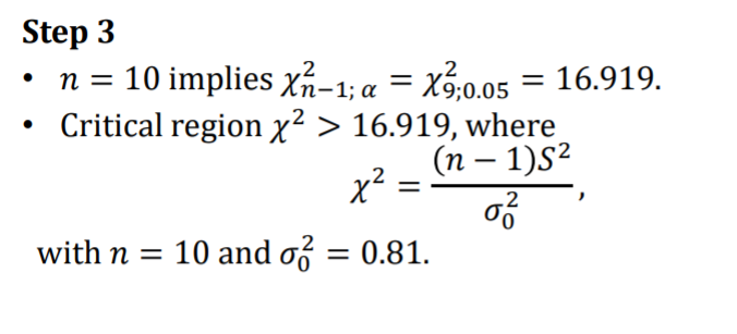
E.g 1
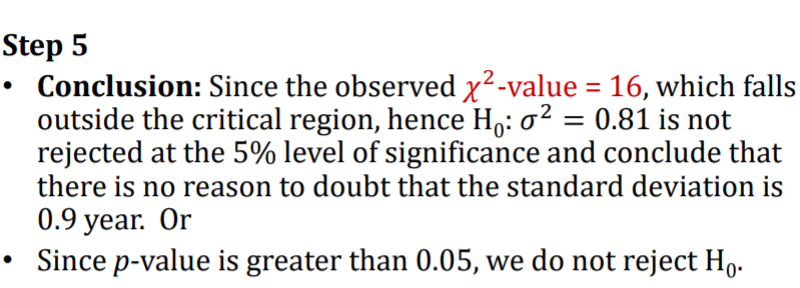
- Batt has a sd 0.9 year
- Random sample of 10 of these batt have sd of 1.2 years
- Do u think that sigma > 0.9
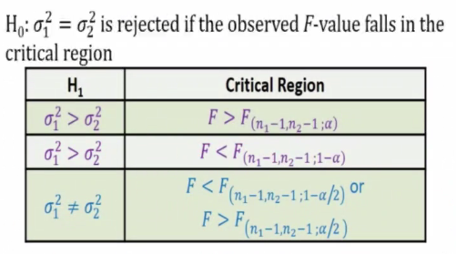
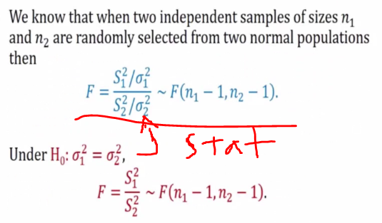
H.T Concerning ratio of variances
Assume:
- Underlying is normal
- Means are unknown
e.g 2
- Mat 1 has 11 (Level of freedom)
- Mat 2 has 9 (Level of freedom)
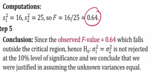
- Mat 1 avg 85 and sd 4
- Mat 2 avg 81 and sd 5
- Test two variance are equal using 0.1 sig
1)
Test sig1 = sig2
3) n1 = 11 n2 =9 implies that F10,8,0.05 = 3.35
- F 8,10;0.05 = 1/3.07 = 0.326
Note: F distribution is a ratio of 2 chi square distribution

