Population and sample

How does each sample’s avg behaves? That is the sampling distribution

The totality of possible outcomes or observation of a surve or experiment is populate
Sample is a subset of population
Every outcome or observation can be recorded as a numerical or categorical value. Thus each member of a population is a value of a random variable.

Finite population

Finite number of elements

e.g

All citizen of singapore
All books in science library

Population is a collection of something that has a value and it can have more than one of these value.

Infinite Population

Infinite is one that consists of an infinitely (Countable and uncountable) large number of elements.

e.g

The results of all possible rolls of a pair of dice
Random digits numbers taken with replacement from a sample space of 10 digits. like {0,1,2,3,4,5,6,7,8,9}

Although they are only 10 distinct integers, there can be a replacement, thus it is infinite

The depths at all conceivable position of a lake

There is infinite number of points

Remark

Some infinite pop are so large that intheory we assume to be infinite such as the pop of lives of a certain type of storage battery.

Random Sampling

Simple random sample

A set of n members takne from a given population is called a sample of size n
A simple random sample of n members is a sample that is chosen in such a way that every subset of n observation of the population has the same prob of being selected

We want to select a sample of 3 from 1,2,3,4,5,6,7,8,9,10,11,12

We can select using 12C3 -> e.g {1,8,9}

Each of these are equally likely of being selected

Sampling from a finite population

Sampling without replacement
- In general, there are NCn samples of size n that can be drawn from a finite population of size N without replacement

Each sample has an equal chance of being selected

p(select) = 1/Ncn

Sampling with replacement
- Using the population {A,B,C,D}, there are 4^2 = 16 samples of size 2

There are N^n sample of size n that can be drawn from a finte pop of size N with replacement

Sampling from an infinite population (with or without)

It wont affect the remaining if you take one out because it is infinite.

E.g 1

15 tosses of a coin with the hypothetical infinite population as the result
If prob of getting heads is the same
15 tosses are independent

-> Therefore, the sample is random

Each of these values are independent and has an even distribution The joint distribution is equal to the product of the joint marginal for each values.

1) same prob of being selected 2) Independent

E.g 3

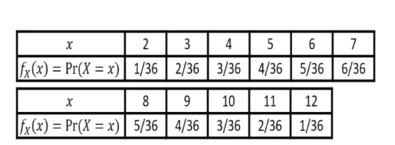
Consider the pop of the sum of all possible rolls of a pair of dice
the population is consider to be infinite
We choose a random sample of size n from a random variable X having probability function given by

is infiite cos we can roll the dice many times

To obtain a random size of size 100, we simply roll the pair of dice 100 times independently under the same conditons
If xi represent the result on the ith roll, we then obtain x1,x2,x100
All these are random variables with the same prob/same distribution as the population variable X

no matter is what roll, the outcome will follow the same distribution

Definition

Let X be random variable with prob distribution
Let x1,x2.. xn be n independent random variables each having the same distribution as X
then x1,x2..xn is called a random sample of size n from a population with distribution fx(x)

Sampling distribution of sample mean

Selecting random sample to elicit infomation about unknown population parameters

e.g we just toss a coin

fx(x) = p^x * (1-p) ^ (1-x) * x

We draw inference from a subset of a population

We want to know the proportion of people in singapore who prefer a certain brand of coffee
A large random sample is then selected from the population and the proportion of this sample favouring the brand of coffee in question is calculated

All these answer being correct or incorrect, they are all answer since we are selecting a random sample

Statistic and sampling distribution

A function of a random sample is call statistic

A function is when we have one value mapped to another value

A statistic is also called a random variable
The prob distribution of a statstic is called a sampling distribution

Sample mean

This is the realisation of the statistic This happen wehen the values in the random sample is observed

E.g 1

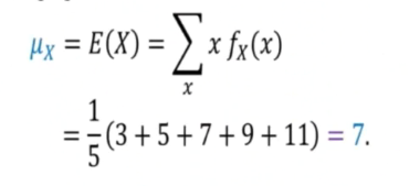
Consider a discrete uniform population
3,5,7,9,11
Population N = 5

Hence, fx(X) = 1/5

The population mean

Note: Mean is not the average, we must use the fomular

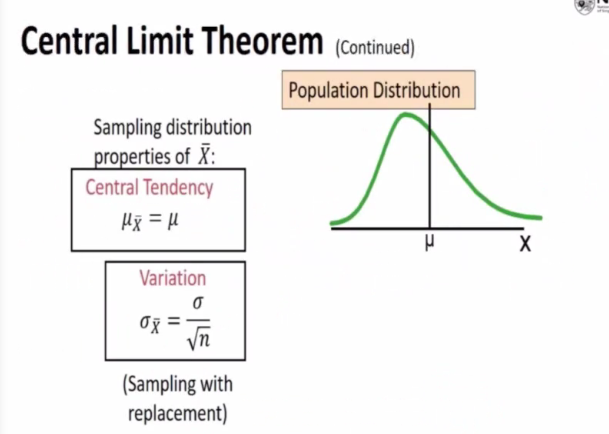
v(xspa) = v(x) / n

E(xpa) = e(x)

The variation of xpa is smaller than the variation of x. Because variance of xspa is v(x) * n. If n is a big number, then the varation of xspa is close to 0 compared to v(x)

Theorem

FOr random samples of size n taken from infinite population or finite with replacement, having population mean (u)and population deviation(sigma)

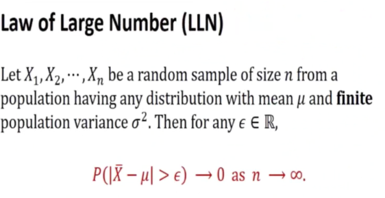
Law of large number

The number is very big

-> Seems to tend to 0 when n is big

Remark:

The sample size increase, the prob that the sample mean differes from the population mean tends to 0

Central Limit theorem and its application

Let x1, x2.. xn be random sample of size n from a population having any distribution with mean u and finite population variance sigma^2

The sampling distribution of the sample mean xspa is approximately normal with mean u and variance sigma^2/n if n is Sufficiently large

Taking a random sample of a million does not mean it will follow this normal distribution -> but that all the mean will follow the approximate normal

e.g If i select one million from a population and ask them a yes or no question. Each individual question be yes or no. How can it follow normal distribution? However, if we take the sample mean, all the xspa will follow the same normal distribution

Big sample size means that the sample mean follow a normal distribution

Theorem

If given a bunch of x which follow N(u,sigma^2), then xspa is N(u,sigma^2/n) regardless of the sample size n

The sum of a1x1…anxn is a linear combination.

The whole expression is an random variable. What is the distribution for this random variable.

Variance is sigma^2/n, this does not require the n to be large. If it is approximately normal, the Xspa is approximately normal as well. N(u,sigma^2/n) regardless of the sample size n

E.g 1

Light bubl have a length of life that is approx normally distributed
Mean equal to 800 hours
SD 40 hrs
Find prob of randomsample of 16 light bulbs will have an avg life of less than 775 hours

Xspa approx ~ N(800, 40^2/16)

Therefore,

It is symmetric about 0, therefore p(z<-0.5) = p(z>2.5). We do not need a graphic calculator

E.g 2

Xspa denote the mean of random sample size 75
Distribution with pdf:

fx(x) = 1 for 0<x<1

What is xspa?

xspa ~N(E(x), V(x)/n)

Find (0.45<xspa<0.55)
It is known that E(X) = 1/2 and v(x) = 1/12

E(Xspa) = E(x)

V(xspa) = V(X) /n

E.g 3

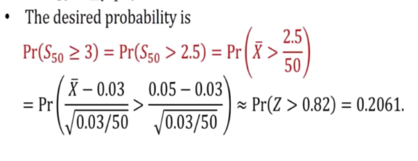
Random sample size 50 from possion distribution with para lamda = 0.03
What is the prob that the sum of the sample will be at least 3 ie p(xspa>=3)

By the theorem, Xspa~N(E(x) , v(x)/n)

E(x) = 0.03 = V(x) due to poisson

Therefore,

Note: Continuity correction is used.

If the sample size is very big, it does not really matter.

E.g 4

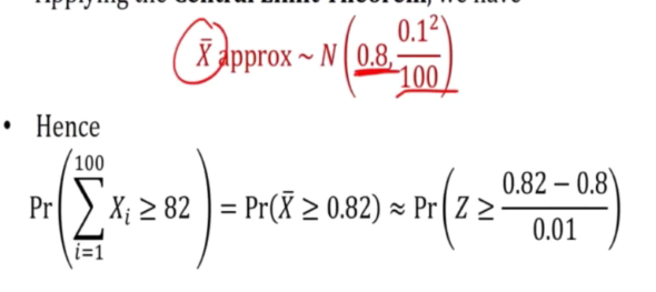
Nicotine content mean= 0.8mg
SD 0.1mg
SOmeone smokes 5 packs (20 cigarettes) per week

-> 5 packs consist of 100 cigarettes -> Let xi denote the nicotine contents of the 100 cigarettes

Applying clt,

This is the same as asking if xspa is greater or equal to 0.82

Sampling distributions of difference of two sample means

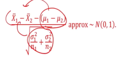
What if we have x1spa and x2spa

Since x1spa and x2spa are approx normally distributed, therefore their differences are also approximately normally distributed.

E.g 1

Tv picture tubes of manufacturer A have a

mean lifetime of 6.5 years
sd of 0.9 years

Manu B have

mean 6
SD - 0.8

What is the prob that a random sample of 36 tubes from A have mean that is at least 1 year more than mean of sample 49 from B?

P(Xspa - Yspa >=1)

Mean is 6.5 - 6 = 0.5
SD = Sqrt((0.81/36) + (0.64/49))

We are not told what is the distribution, we only know the mean, That is why we will approximate the distribution to the normal distribution

Chi square distruution

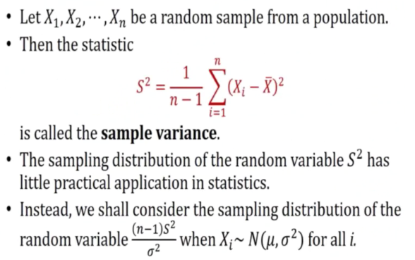
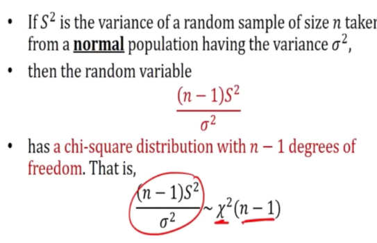
Now we are talking about how sample variance behaves

This will follow the ~x^2(n-1) distribution.

This is the PDF for y:

Y is defined to have a chi square distribution with n degress of freedom denoted by X^2(n) Where n is a positive integer and R(.) is the gamma function

![2334_5_15.PNG(/NUSCSMODS/img/2334_5_15.PNG)

Properties

Y~x^2(n), then E(Y) = n and V(Y) = 2n
For large n, X^2(n) approx ~ N(n,2n)
If Y1..Yk are independent chi sqaer random cariabe with n1..nk degress of freedom respectabl, then the sum of y1 to yk has a chi square distribution with n1 + ..nk degress of freedom

Theorem

If X~N(0,1), then X^2 ~X^2(1) Where x is (y-u)/sigma

Sampling distribution of (n-1)S^2 /

t-distribution

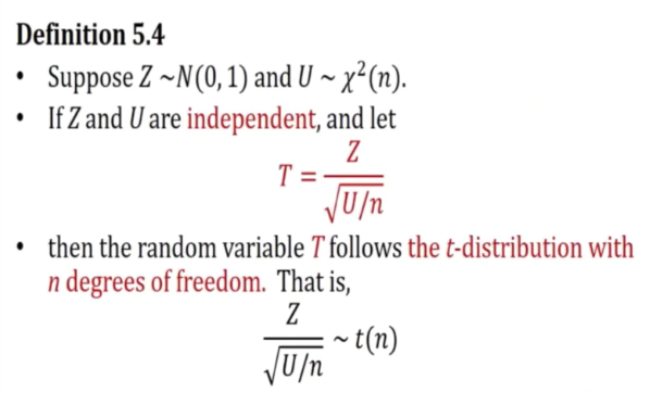
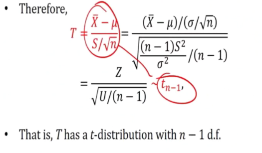
Z is Xspa - u / (sigma/sqrt(n)) ~N(0,1)

The final is Xspa - u / (s/sqrt(n)) which is the t distribution

This t distribution is consider as the ratio of 2 random variables, x and z.

Properties of t-distribution

Resembles a graph of a sd distribution
As n tend to infinite, it looks like normal distribution

E.g 1

Light bubl burn on avg 500 hrs
Test 25 bubls each month
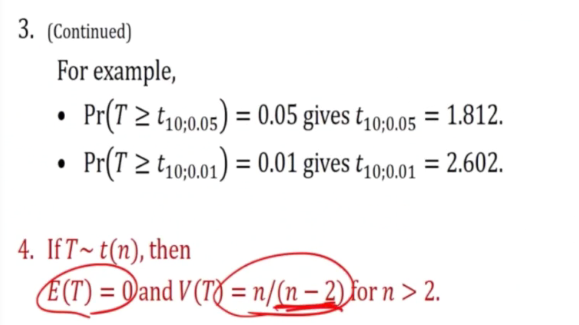
Computed t values falls between -t24;0.05 and t24;0.05
What conclusion should be drawn from a sample that has a mean Xspa 518 hours and sd s = 40?

The chance that falls between t(24) and betwen -1.71 and 1.71, what is the probability that it falls within this area in the graph.

Assume that the distribution of burning times in hours is approx normal

if u =500 then t = (518-u)/(40/5) = (519-500)/8 = 2.25 > 1.711

In this case, we do not believe what the manufacturer claim as u is > 500.

F-distribution

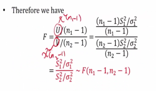
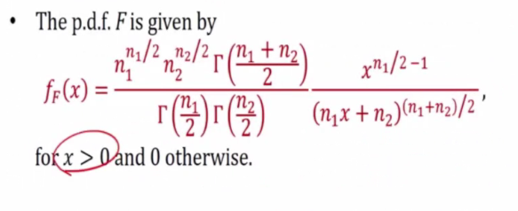
Let U and V be independent random variables having X^2(n1) and X^2(n2) respectively.

Definition

E.g 1

Sppose random samples of size n1 and n2 are selected from 2 normal pop with varaince of sigma1 and sigma2 respectively

We are interested in finding if the 2 sample population have the same variance. Thus we will use this

Theorem

If F~F(n,m) then 1/F ~ F(m.n)

We are just taking the reciprocol since it is a ratio. We need to swap the degrees of freedom
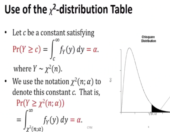
The table gives the values of F(n1,n2;a) such that P(F>F(n1,n2;a)) = a

E.g

F(5,4;0.05) = 6.26 means p(f>6.26) = 0.05 where f~F(5,4)
F(4,5;0.025) = 7.39 means P(F>7.39) = 0.025 where F ~ F(4,5)

Theorem

P(W>a) = 1 - alpha
P(1/w < 1.a) = 1 - alpha
P(1/w > 1.a) = alpha

E.g 2

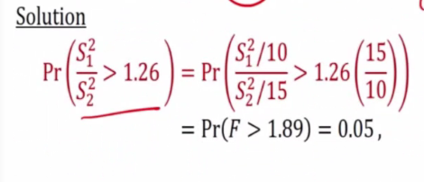
S1^2 and S2^2 be sample variances of independent sample of size n1 = 25 and n2 = 31
Normal population with variance 10 and 15 respectively
Find P(S1^2 / S2^2 > 1.26)